Crash-course in Quarto
What is Quarto?
Quarto is a plain-text system for writing documents that can include code (R, Python, etc.). You write a .qmd file and render it into HTML (this unit will use HTML). Quarto handles the formatting, runs your code, and inserts the results.
A Quarto document usually has:
- A header (between
---lines) using YAML notation - The body: your text + headings + code blocks
Example YAML header that produces html format output (pdf and docx are also possible):
---
title: "My analysis"
author: "My Name"
format: html
---
The body text comes after the YAML header.
Here’s a minimal Quarto document that produces an html file.
---
title: "My analysis"
author: "My Name"
format: html
---

Hello, world!
Headings and text formatting
Headings
Use # symbols; different numbers of # for different headling levels. You need an empty line after each heading.
# Main heading

Here's some main text. Note the line directly above is empty.

## Subheading

Here's some more text in a subsection. Note again the line directly above is empty.

### Sub-subheading

Here's some more text in a sub-subsection. Line directly above is empty still!
Italics and bold
*italic*produces italic text, e.g. Escherichia coli**bold**produces bold text, e.g. important***bold and italic***produces bold and italic text, e.g. very important
Inline code
Use backticks ` to indicate code within a sentence.
The `mean(x)` function calculates the mean of the input vector `x`.Code blocks (R)
Quarto can both show and execute R code blocks within the document. You can include a code block like this:
```{r}
library(tidyverse)
data <- read_csv("my_data.csv")
```- Code runs during rendering.
- Output (tables, plots, messages) appears in the HTML.
You can set options to control what is shown:
```{r}
#| echo: false
#| message: false
# This code would run but not show the code or messages from loading tidyverse
library(tidyverse)
data <- read_csv("my_data.csv")
```
Figures made by R
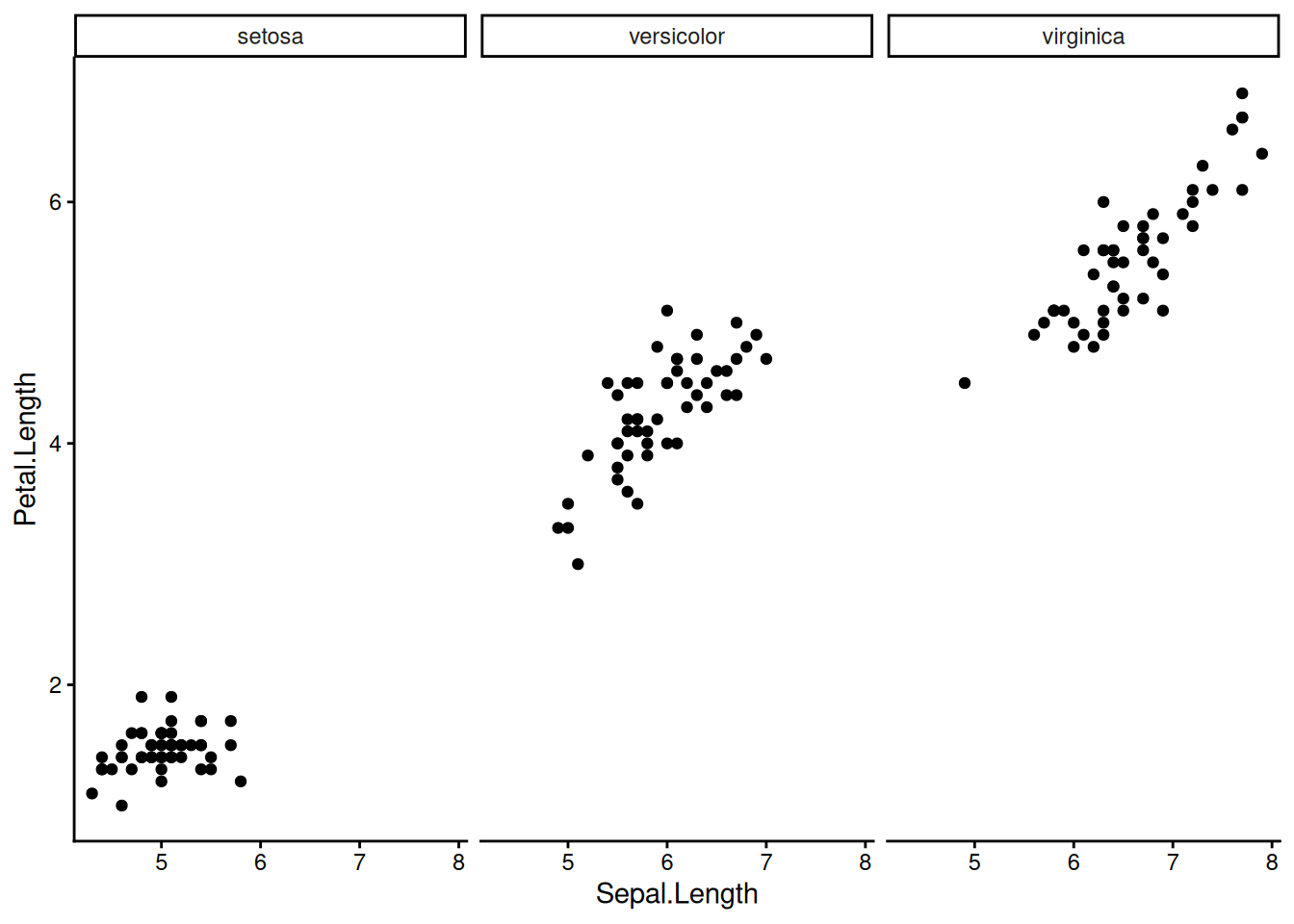
Plots appear automatically when code produces them:
```{r}
#| message: false
#| eval: false
ggplot(iris, aes(x = Sepal.Length, y = Petal.Length)) +
  geom_point() +
  facet_grid(~Species) +
  theme_classic()
```
You can control figure size (NB: sizes are in inches):
```{r}
#| eval: false
#| fig-width: 6
#| fig-height: 4
ggplot(data, aes(x, y)) +
  geom_point()
```Tables
R will print tibbles as they would appear in the console.
```{r}
# Example using the iris dataset

# First convert iris to a tibble
iris_tibble <- as_tibble(iris)

# Print iris_tibble
iris_tibble
```
# A tibble: 150 × 5
Sepal.Length Sepal.Width Petal.Length Petal.Width Species
<dbl> <dbl> <dbl> <dbl> <fct>
1 5.1 3.5 1.4 0.2 setosa
2 4.9 3 1.4 0.2 setosa
3 4.7 3.2 1.3 0.2 setosa
4 4.6 3.1 1.5 0.2 setosa
5 5 3.6 1.4 0.2 setosa
6 5.4 3.9 1.7 0.4 setosa
7 4.6 3.4 1.4 0.3 setosa
8 5 3.4 1.5 0.2 setosa
9 4.4 2.9 1.4 0.2 setosa
10 4.9 3.1 1.5 0.1 setosa
# ℹ 140 more rowsFor prettier formatted tables (advanced, not required for assessment):
```{r}
library(knitr)
kable(head(iris_tibble))
```| Sepal.Length | Sepal.Width | Petal.Length | Petal.Width | Species |
|---|---|---|---|---|
| 5.1 | 3.5 | 1.4 | 0.2 | setosa |
| 4.9 | 3.0 | 1.4 | 0.2 | setosa |
| 4.7 | 3.2 | 1.3 | 0.2 | setosa |
| 4.6 | 3.1 | 1.5 | 0.2 | setosa |
| 5.0 | 3.6 | 1.4 | 0.2 | setosa |
| 5.4 | 3.9 | 1.7 | 0.4 | setosa |
Lists
You can make ordered/numbered lists and unordered/bullet point lists like this. Note that you need an empty line before and after a list. Ordered list:
<-- empty line!
1. First
2. Second
3. Third
<-- empty line!
Unordered list:
<-- empty line!
- item
- item
- item
<-- empty line!
Links
You can insert links into your document.
Raw link, e.g. http://example.com:
<http://example.com>Formatted link, e.g. visit Example.com:
[visit Example.com](http://example.com)Images
Images not created in R can also be included:

With alt text:
Citations using footnotes
You can make simple citations using footnotes.
In the text:
Here is some text with a citation[^paper1].At the end of the document:
[^paper1]: John Doe, "Frogs," *Journal of Amphibians* 44 (1999)
[^paper2]: Susan Smith, "Flies," *Journal of Insects* (2000)
[^paper3]: Susan Smith, "Bees," *Journal of Insects* (2004)
(Advanced) Citations with a bibliography
For complex documents, you can include a references list. (This is not required for the assessment.)
If you use a .bib file or Zotero, add it in the YAML:
---
title: "My report"
format: html
bibliography: references.bib
---
Then, in the text:
[@smith2000]   # in brackets
@smith2000     # no brackets
In the visual editor, you can also insert references into your bibliography file using their DOI @10.1099/mic.0.001534.
More information:
https://quarto.org/docs/authoring/citations.html
https://quarto.org/docs/visual-editor/technical.html#citations
Rendering your document
In RStudio:
- Create a new Quarto file (File>New File>Quarto Document) or open your existing
file.qmdfile. - Click the Render button (or Shift-Command/Command-K).
This produces file.html in the same folder where your file.qmd is saved. You can open this file in any web browser (e.g. Chrome, Firefox, Edge).
Common pitfalls
- Missing fences: R code must be in ‘fenced’ code blocks (three backticks, ```) for Quarto to run it.
- File paths: Quarto runs from the project directory, so
"data/myfile.csv"must exist there.
- Missing empty lines: headers and lists need empty lines before and after.
- Header formatting: The YAML header is sensitive to spacing and indentation. Keep colons followed by a space, and do not use tabs.
Useful references
- Quarto getting started: https://quarto.org/docs/get-started/
- R-focused overview: https://r4ds.hadley.nz/quarto.html
Comments and organisation
Add comments inside R code blocks: