Hypothesis testing

From questions to statistical decisions

BIOL33031 / BIOL65161

Why we need hypothesis testing

We use hypothesis testing to assess whether the pattern we see in our data is unlikely to have arisen by random chance alone.

For example:

• Do males and females of a given species differ in body mass?
  
• Does an antibiotic reduce bacterial growth compared with a control?

Because biological data are variable, we can’t trust a single mean difference — we need a framework to decide when an effect is convincing.

In biology, variation is everywhere — individuals differ, experiments fluctuate, and sampling introduces noise.
Hypothesis testing provides a structured way to ask whether a pattern could have arisen by chance alone.
We don’t want to over-interpret small fluctuations, so this framework gives us a level of confidence before drawing conclusions.

The idea of a null hypothesis

The null hypothesis (H₀) represents the idea of no real effect.

• It represents what we’d expect if any difference is just due to random noise.
• We compare it with the alternative hypothesis (H₁), which suggests a real effect exists.

If our question is something like, “Does body mass differ between and females?” our null and alternative hypotheses would be:

• H₀: Mean body mass is the same for both sexes.
  
• H₁: Mean body mass differs between sexes.

This is known as a “two-tailed hypothesis test”: we are interested in whether our data differ than we expected under the null hypothesis, i.e. is either larger or smaller (we don’t care which).

The idea of a null hypothesis

The null hypothesis (H₀) represents the idea of no real effect.

Our question could also be “Is the flipper length of males larger than females?”

• H₀: Male mean flipper length is equal to or less than female mean flipper length.
• H₁: Male mean flipper length is larger than female flipper length.

Or, “Is the bill length of Gentoo penguins shorter than of Chinstrap penguins?”

• H₀: Mean bill length for Gentoo penguins is equal to or longer than for Chinstrap penguins.
• H₁: Mean bill length for Gentoo penguins is shorter than for Chinstrap penguins.

These are both examples of “one-tailed hypothesis tests”: we are interested in testing whether are data are either larger, or smaller, than expected under the null hypothesis–and the direction of the difference matters.

We start every test with the assumption that there’s no real difference — that’s the null hypothesis.
Then we collect data and see how far the results deviate from that assumption.
If the data look very unlikely under H₀, we begin to doubt it and consider the alternative.

The test statistic

To answer that question, we calculate a test statistic — a number that captures how different our observed data are from what we’d expect under H₀.

Different tests use different statistics:

Test	Typical data type	Statistic
t-test	Comparing means	t-value
χ² test	Counts/frequencies	χ² value
correlation	Relationship between variables	r

Large values of the statistic usually mean the data deviate strongly from H₀.

The test statistic is like a summary of how likely we are to have observed our data if the the null hypothesis was true.
Each statistical test converts your raw data into a single value that’s easy to compare against a theoretical distribution.
We then see whether that value is extreme enough to make us doubt H₀.

The p-value

The p-value is the probability of seeing a result as extreme as ours if the null hypothesis were true.

• A small p-value means our data are unlikely under H₀.
  
• A large p-value means the data are compatible with H₀.

Conventionally, we use a threshold (α), often 0.05:

• If p < 0.05: we reject H₀ (evidence for an effect).
  
• If p ≥ 0.05: we fail to reject H₀ (no evidence of an effect).

Note: we never “accept” or “prove” H₀ — we only fail to reject it.

This is the heart of hypothesis testing.
A p-value tells us how extreme our data are if the null were actually true.
A small p-value suggests the data don’t fit the null well — but it doesn’t tell us the probability that H₀ is true.

It’s important to note that we never “accept” or “prove” the null hypothesis, we only fail to reject it.

Visualisng p-values: two-tailed hypotheses

Imagine the distribution of outcomes expected under H₀.
Most outcomes cluster near the centre (small differences), but extreme outcomes are rare.

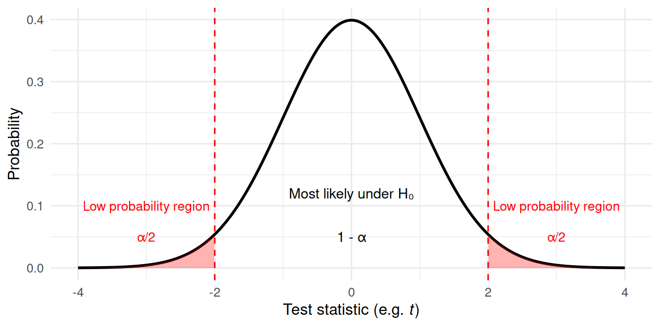
If our test statistic falls in the red region (p < 0.05), we reject H₀.

This figure shows how hypothesis testing works visually.
If your test statistic lies within the centre region, the result is common under H₀.
But if it’s in the tails (the red regions) the result would be unexpected if H₀ were true, so we reject it.

Visualising p-values: one-tailed hypotheses

When our alternative hypothesis predicts a specific direction of effect, we only consider one tail of the distribution.

NULL

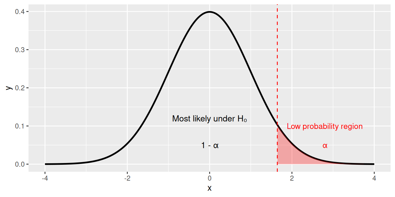
If our test statistic falls in the red region (p < 0.05), we reject H₀ in favour of the directional alternative.

In a one-tailed test, we only look for an effect in one direction. The entire α (e.g. 0.05) is concentrated in a single tail, so the rejection region is larger compared with each tail of a two-tailed test. This makes the test more sensitive to effects in the predicted direction — but unable to detect effects in the opposite direction.

Example: Antibiotic test

Suppose we grow bacteria with and without an antibiotic:

Treatment	Mean OD600	SD	n
Control	0.80	0.05	5
Antibiotic	0.62	0.06	5

We perform a t-test and get p = 0.01.

Interpretation:

• If there were no real difference in growth, data like this would occur only about 1% of the time.
  
• Therefore, we reject H₀ — the antibiotic likely reduces growth.

It helps to ground the concept in a biological example.
Here we compare bacterial growth with and without antibiotic treatment.
Because the p-value is small, we conclude that the difference is unlikely to be due to random variation alone.

Type I and Type II errors

Statistical testing involves probabilities — so mistakes can happen.

Error type	What happens	Probability
Type I	Reject H₀ when it’s actually true (false positive)	α (e.g. 0.05)
Type II	Fail to reject H₀ when it’s actually false (false negative)	β

Reducing α makes Type I errors rarer, but increases Type II errors.
We can reduce both by collecting larger samples (increasing power).

No test is perfect.
If we’re too strict, we might miss real effects (Type II).
If we’re too lenient, we’ll claim effects that aren’t real (Type I).
The solution is usually to increase our sample size — more data means fewer mistakes.

Statistical power

Power = probability of correctly rejecting a false null hypothesis (1 − β).

Power increases with:

• Larger sample size
  
• Larger true effect size
  
• Lower variability
  
• Higher α (though that increases false positives)

Power analysis helps plan experiments that are sensitive enough to detect real effects.

Power is about the sensitivity of a test.
A low-power experiment might miss real biological patterns, leading to misleading “no effect” results.
Planning with power in mind ensures experiments can detect effects that matter.

Statistical vs biological significance

Even a very small difference can be “statistically significant” if n is large.
But that doesn’t mean it’s biologically meaningful.

Example:

• 0.2 g difference in penguin body mass might be statistically significant but trivial biologically.

Always interpret results in context: does the difference matter biologically, or just statistically?

Statistical significance isn’t the same as importance.
We care about whether the effect size makes a meaningful biological difference.
Always connect your statistical findings back to the biology.

Common misunderstandings

• A p-value does not tell us the probability that H₀ is true.
  
• Non-significant results don’t prove there is “no effect.”
  
• Statistical significance ≠ importance.
  
• Multiple testing inflates false positives — corrections are needed.

Students often misinterpret p-values and non-significant results.
It’s worth repeating: “not significant” doesn’t mean “no effect.”
And when testing many hypotheses, the chance of false positives rises — that’s where corrections like Bonferroni or FDR come in.

Reporting results

Always report:

• The test used (e.g. Welch’s t-test)
  
• The test statistic (t, F, χ², etc.)
  
• Degrees of freedom and p-value
  
• Optionally, effect size and confidence interval

Example:

Welch’s t-test: t(8) = 3.12, p = 0.014; mean difference = 0.18 ± 0.06 (95% CI).

Good reporting is about transparency.
Anyone reading your paper should know what test was used, what the result was numerically, and how big the effect was.
Including confidence intervals helps readers judge precision.

Recap & next steps

• Hypothesis testing compares observed data with what we’d expect under no effect.
  
• The p-value measures how extreme our data are under H₀.
  
• We make decisions using a threshold (α), but always with caution.
  
• Interpretation requires both statistical reasoning and biological insight.

In the next practical session, you’ll learn how to apply t-tests in R, interpret p-values and confidence intervals, and practice describing results clearly in text.

Summarise key ideas before finishing.
Remind students that hypothesis testing is a tool, not a truth machine — it helps guide inference but must be interpreted in context.