Data wrangling

BIOL33031/BIOL65161

Data wrangling

Welcome to our session on data wrangling. This week we’ll look at how we take raw biological data and turn it into something we can actually analyse. Real datasets are rarely perfect — they come with missing values, messy names, or too many columns. Our job is to wrangle them into a clean, tidy form that R can work with.

What is data wrangling?

When we collect biological data, it never arrives perfectly polished. Files might have missing values, inconsistent names, or more information than we really need.

Before we can analyse or visualise, we first have to wrangle our data into a form that both we, and R, can understand. Part of this also involves checking if there are any problems with the data (like missing values), or anything unexpected that might be confusing (like columns with unintuitive names).

The word wrangle can mean either “to have an argument that continues for a long time” (chiefly UK), or “to take care of, control, or move large animals, often with difficulty or coercion” (chiefly North American). In dealing with biological data, either definition can sometimes feel appropriate!

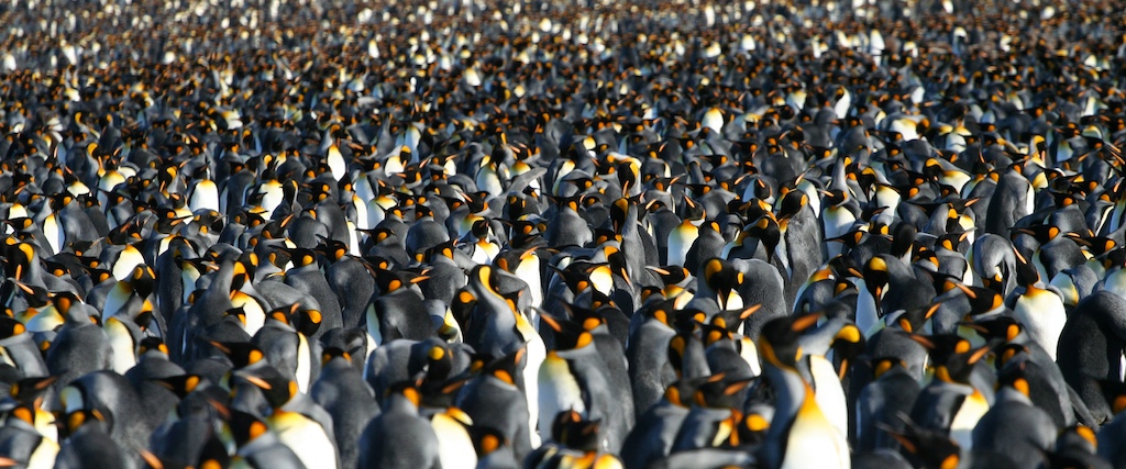
“King Penguin Colony” (Aptenodytes patagonicus) by Scott Henderson, CC BY-NC-SA 2.0

When we talk about wrangling, we mean cleaning, reshaping, and preparing data. It’s the step between collecting your data and analysing it. Sometimes it feels like arguing endlessly with your data, and other times like herding stubborn animals — both meanings of “wrangle” are pretty accurate! But once the data are tamed, everything that follows becomes easier.

Remember tibbles?

In the first session, we made some tibbles by hand to see how R stores data.
A tibble is just a table where:

• Each column is a variable (e.g. species, sepal length)
  
• Each row is an observation (e.g. one plant)
  
• Each cell is a single value (i.e. the measurement of that variable for that individual)

Example from last time:

library(tidyverse)

plants <- tibble(
  treatment = c("control", "fertilised", "control"),
  height_cm = c(15, 20, 13),
  survival = c(TRUE, TRUE, FALSE)
)

plants

Now, it would be a colossal waste of time if we had to write out each tibble manually!
Typically in R, we read in data from files on our computer or from the internet.

You might remember that in R we store data in tibbles — tidy little tables. Each column is a variable, each row is an observation, and each cell holds one value. For example, one column could be “species”, another “flipper length”, and each row would be a single penguin. Writing these by hand would be ridiculous — so we normally import data from files instead of typing them out manually.

Telling R where to look for data

• Every time R looks for a file, it needs to know where to look.
  
• The simplest way to do this is to set your working directory, and keep your .R scripts and data files together in the same place
• Imagine your computer as a giant house 🏡. The working directory is the room you’re currently in. R will look for files within that room. If the file is in another room, R won’t find it unless you give the full address.

You can check or set the working directory with getwd() and setwd():

getwd()                 # shows where you are now
setwd("path/to/folder") # moves R to another room

You can also set the working directory using the menu:
“Session > Set Working Directory > Choose Directory…”

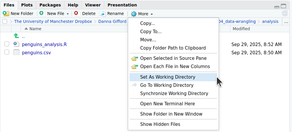
Or, you can use the Files tab on the right:

Before we can import data, R needs to know where the file lives. That’s what the working directory is. Imagine your computer as a big house and R as standing in one room — that room is your working directory. If your data are in another room, R can’t see them unless you give it the full address. You can check where you are with getwd() and move rooms with setwd(), or just use the Files tab or Session menu in RStudio.

Palmer penguins dataset 🐧

Let’s have a look at some common data wrangling steps using real data.

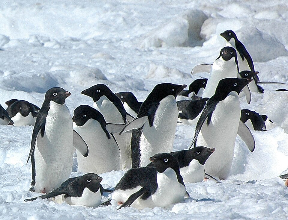
The palmerpenguins dataset¹ contains size measurements for 3 penguin species observed between 2007‒2009 in the Palmer Archipelago, Antarctica, by Dr. Kristen Gorman with the Palmer Station Long Term Ecological Research Program.

If you’re following along in R, please download penguins.csv and save it to your working directory.

Sampling context: (a) Antarctica. (b) Antarctic peninsula. (c) Islands where penguins were sampled: Dream, Torgersen, and Biscoe.²

To practise, we’ll use the Palmer Penguins dataset. It contains measurements from three species of penguins collected in the Palmer Archipelago, Antarctica, between 2007 and 2009 by Kristen Gorman and colleagues. If you’re following along, download the file penguins.csv and save it in your working directory. It’s a perfect example of tidy, real biological data.

1. Horst AM, Hill AP, Gorman KB (2020). palmerpenguins: Palmer Archipelago (Antarctica) penguin data. R package version 0.1.0. https://allisonhorst.github.io/palmerpenguins/. Data are available by CC-0 license in accordance with the Palmer Station LTER Data Policy and the LTER Data Access Policy for Type I data, part of the US Long Term Ecological Research Network.

2. Original publication: Gorman KB, Williams TD, Fraser WR (2014). Ecological sexual dimorphism and environmental variability within a community of Antarctic penguins (genus Pygoscelis). PLoS ONE 9(3):e90081. https://doi.org/10.1371/journal.pone.0090081.

Importing data

Most of the time, our data will be stored in CSV files (comma-separated values).
These are simple text files that can be read by almost any program.

In the tidyverse, we use read_csv()¹:

library(tidyverse)

# First set working directory to where your file is saved. It looks slightly different on different systems:
setwd("C:/Documents/04_data-wrangling/analysis") # Windows
setwd("/Users/danna/04_data-wrangling/analysis") # Mac
setwd("/home/danna/04_data-wrangling/analysis")  # Linux

# Loading the data using read_csv():
# From a file saved on your computer in your working directory
penguins <- read_csv("penguins.csv")

# From a folder called 'data' within your working directory (a 'relative path')
penguins <- read_csv("data/penguins.csv")

# From a file saved somewhere else on your computer (an 'absolute path')
penguins <- read_csv("C:/Documents/data/penguins.csv")              # Windows
penguins <- read_csv("/home/username/Documents/data/penguins.csv")  # Mac
penguins <- read_csv("/Users/username/Documents/data/penguins.csv") # Linux

# Directly from a URL
penguins <- read_csv("https://raw.githubusercontent.com/allisonhorst/palmerpenguins/master/inst/extdata/penguins.csv")

Most datasets come as CSV files — comma-separated values. They’re plain text and easy to open in almost any software. In the tidyverse we use read_csv() to import them. You can read a file from your computer, from a “data” folder, or even directly from a URL. Whichever method you use, read_csv() gives you a tibble containing your data, ready to explore.

1. NB: It is important that you use read_csv() throughout the unit. Base R uses read.csv(), which imports data in a slightly different way.

Meeting the tibble

When you use read_csv(), R gives you a tibble, just like the ones we wrote by hand.

Typing in the name of the tibble and pressing Ctrl+Enter (Windows/Linux) or Cmd+Enter (Mac) will print the first 10 rows to the Console window:

penguins

# A tibble: 344 × 8
   species island    bill_length_mm bill_depth_mm flipper_length_mm body_mass_g
   <fct>   <fct>              <dbl>         <dbl>             <int>       <int>
 1 Adelie  Torgersen           39.1          18.7               181        3750
 2 Adelie  Torgersen           39.5          17.4               186        3800
 3 Adelie  Torgersen           40.3          18                 195        3250
 4 Adelie  Torgersen           NA            NA                  NA          NA
 5 Adelie  Torgersen           36.7          19.3               193        3450
 6 Adelie  Torgersen           39.3          20.6               190        3650
 7 Adelie  Torgersen           38.9          17.8               181        3625
 8 Adelie  Torgersen           39.2          19.6               195        4675
 9 Adelie  Torgersen           34.1          18.1               193        3475
10 Adelie  Torgersen           42            20.2               190        4250
# ℹ 334 more rows
# ℹ 2 more variables: sex <fct>, year <int>

Adélie penguin (Pygoscelis adeliae) near Snow Hill, Antarctica (2007). Source: Wikimedia.

After you import, just type the name of the tibble to see the first few rows. You should see columns for species, island, bill length, bill depth, flipper length, body mass, sex, and year — one row per penguin. This quick peek confirms the data loaded properly. It’s also a good habit to always look at your data before doing anything else.

Looking at the data

Once you have loaded your data, you should check to see if it looks the way you think it should.
There are a few quick ways to peek. You should type these into the Console window.

head(penguins)      # shows the first few rows

# A tibble: 6 × 8
  species island    bill_length_mm bill_depth_mm flipper_length_mm body_mass_g
  <fct>   <fct>              <dbl>         <dbl>             <int>       <int>
1 Adelie  Torgersen           39.1          18.7               181        3750
2 Adelie  Torgersen           39.5          17.4               186        3800
3 Adelie  Torgersen           40.3          18                 195        3250
4 Adelie  Torgersen           NA            NA                  NA          NA
5 Adelie  Torgersen           36.7          19.3               193        3450
6 Adelie  Torgersen           39.3          20.6               190        3650
# ℹ 2 more variables: sex <fct>, year <int>

glimpse(penguins)   # a sideways summary of all columns

Rows: 344
Columns: 8
$ species           <fct> Adelie, Adelie, Adelie, Adelie, Adelie, Adelie, Adel…
$ island            <fct> Torgersen, Torgersen, Torgersen, Torgersen, Torgerse…
$ bill_length_mm    <dbl> 39.1, 39.5, 40.3, NA, 36.7, 39.3, 38.9, 39.2, 34.1, …
$ bill_depth_mm     <dbl> 18.7, 17.4, 18.0, NA, 19.3, 20.6, 17.8, 19.6, 18.1, …
$ flipper_length_mm <int> 181, 186, 195, NA, 193, 190, 181, 195, 193, 190, 186…
$ body_mass_g       <int> 3750, 3800, 3250, NA, 3450, 3650, 3625, 4675, 3475, …
$ sex               <fct> male, female, female, NA, female, male, female, male…
$ year              <int> 2007, 2007, 2007, 2007, 2007, 2007, 2007, 2007, 2007…

View(penguins)   # a spreadsheet-style viewer (but you cannot edit values).

🟦 Looking at the data

There are a few handy ways to inspect it. head() shows the first few rows. glimpse() gives a sideways summary of all the columns and their data types. And View() opens a spreadsheet-style viewer in RStudio — useful for spotting issues, though you can’t edit values there. Always take a moment to check that the data look as expected.

Data types

In the head() and glimpse() output above, you’ll notice that each column has a designation <abc> either below or beside it. These correspond to the “type” of data each column contains. The main data types you will encounter are listed below:

• <chr> means character, which is text or a mixture of text, numbers & punctuation.
  
• <fct> means factor, a special type of text where the levels are pre-defined (e.g. sex).
  
• <dbl> means numbers with decimals, double, a type of numeric.
  
• <int> means whole numbers, integer, another type of numeric.
  
• <lgl> means logical, TRUE/FALSE values (not shown here).
  
• <date> means calendar dates (also not shown here).

This is different from Excel. You should only put data of the same type together in a single column. If you mix data types, it will default to character.

In the output from head() or glimpse(), you’ll see labels like , , or . These are the data types: for character, or text for factor, used for categories like “male” or “female” for numbers with decimals for whole numbers for logical, TRUE or FALSE R behaves differently depending on these types, so make sure each column has the right one.

Tidy data

Now that we know what our data look like, let’s talk about tidy data.

What is tidy data?

A huge amount of effort in analysis goes into cleaning data so that it’s usable. Tidy data gives us a simple, consistent structure that makes analysis, modelling, and visualisation easier.

In tidy data:

• Each variable forms a column
  
• Each observation forms a row
  
• Each value is a cell.

Our penguins dataset is already tidy:

# A tibble: 344 × 6
   species island    bill_length_mm bill_depth_mm sex     year
   <fct>   <fct>              <dbl>         <dbl> <fct>  <int>
 1 Adelie  Torgersen           39.1          18.7 male    2007
 2 Adelie  Torgersen           39.5          17.4 female  2007
 3 Adelie  Torgersen           40.3          18   female  2007
 4 Adelie  Torgersen           NA            NA   <NA>    2007
 5 Adelie  Torgersen           36.7          19.3 female  2007
 6 Adelie  Torgersen           39.3          20.6 male    2007
 7 Adelie  Torgersen           38.9          17.8 female  2007
 8 Adelie  Torgersen           39.2          19.6 male    2007
 9 Adelie  Torgersen           34.1          18.1 <NA>    2007
10 Adelie  Torgersen           42            20.2 <NA>    2007
# ℹ 334 more rows

This also ensures different variables measured on the same observation always stay together.

Tidy data have a simple structure: each variable in its own column, each observation in its own row, and each value in its own cell. Our penguins data already follow this tidy format, which is why they’re so pleasant to work with. Tidy data make analysis, modelling, and plotting consistent across the tidyverse.

Tidying ‘untidy’ data

Untidy data are arranged in any other way, e.g, when column names are actually values, or when several variables are crammed into one column. Here’s some untidy data on Weddell seals, which also live in Antarctica.

Each column represents a combination of variable and year, so the dataset is not tidy — the years are stored as column headers.

weddell <- tibble(
  seal_id = c("W01", "W02", "W03", "W04", "W05"),
  length_2022 = c(260, 250, 270, 255, 265),
  weight_2022 = c(420, 390, 450, 410, 430),
  length_2023 = c(265, 253, 275, 260, 270),
  weight_2023 = c(430, 400, 460, 420, 440)
)

weddell

# A tibble: 5 × 5
  seal_id length_2022 weight_2022 length_2023 weight_2023
  <chr>         <dbl>       <dbl>       <dbl>       <dbl>
1 W01             260         420         265         430
2 W02             250         390         253         400
3 W03             270         450         275         460
4 W04             255         410         260         420
5 W05             265         430         270         440

This layout hides the meaning of the data:

• Year is buried in the column names
• Each row mixes multiple observations (2022 and 2023) for the same seal

But not all datasets you’ll come across are in tidy form. Let’s look at example. Here’s some untidy data on Weddell seals, which also live in Antarctica. This dataset is untidy because the variable ‘year’ is embedded in the column name. Also, each row contains multiple observations for the same seal. This kind of layout is awkward to analyse because the meaning is hidden in the structure.

Making it tidy

We can tidy the seal data by turning those year-specific columns into variables for year, length, and weight.

weddell_tidy <- weddell |>
  pivot_longer(
    cols = starts_with(c("length", "weight")),
    names_to = c(".value", "year"),
    names_sep = "_"
  )
weddell_tidy

# A tibble: 10 × 4
   seal_id year  length weight
   <chr>   <chr>  <dbl>  <dbl>
 1 W01     2022     260    420
 2 W01     2023     265    430
 3 W02     2022     250    390
 4 W02     2023     253    400
 5 W03     2022     270    450
 6 W03     2023     275    460
 7 W04     2022     255    410
 8 W04     2023     260    420
 9 W05     2022     265    430
10 W05     2023     270    440

Now each row is a single observation: one seal, in one year, with one set of measurements

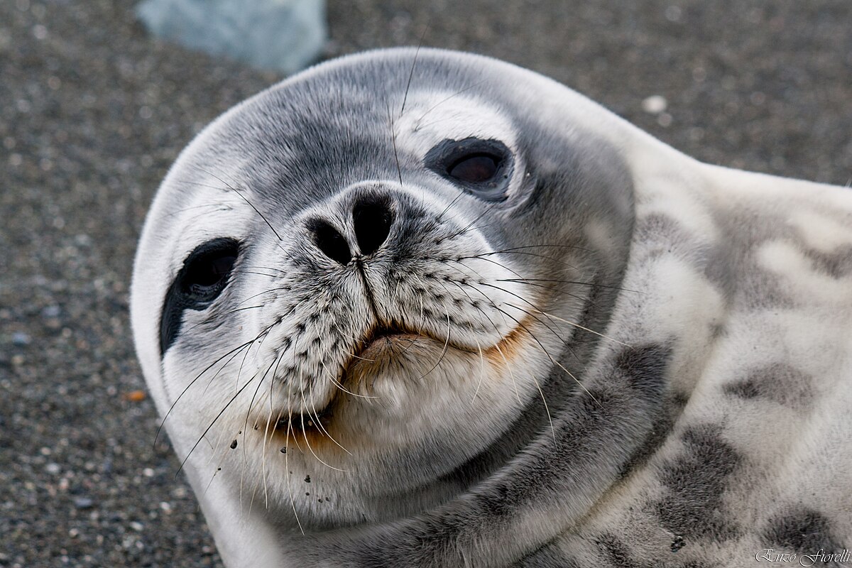
Weddell seal (Leptonychotes weddellii). Image taken by enzofloyd CC-BY-SA 3.0

We can fix that using pivot_longer(). It takes those year-specific columns and turns them into proper variables: one for year, one for length, and one for weight. Now each row represents one seal, in one year, with one set of measurements. That’s the tidy structure we want, and it makes future analyses much easier.

Cleaning and preparing for analysis

Let’s return to our penguins data.

# A tibble: 344 × 8
   species island    bill_length_mm bill_depth_mm flipper_length_mm body_mass_g
   <fct>   <fct>              <dbl>         <dbl>             <int>       <int>
 1 Adelie  Torgersen           39.1          18.7               181        3750
 2 Adelie  Torgersen           39.5          17.4               186        3800
 3 Adelie  Torgersen           40.3          18                 195        3250
 4 Adelie  Torgersen           NA            NA                  NA          NA
 5 Adelie  Torgersen           36.7          19.3               193        3450
 6 Adelie  Torgersen           39.3          20.6               190        3650
 7 Adelie  Torgersen           38.9          17.8               181        3625
 8 Adelie  Torgersen           39.2          19.6               195        4675
 9 Adelie  Torgersen           34.1          18.1               193        3475
10 Adelie  Torgersen           42            20.2               190        4250
# ℹ 334 more rows
# ℹ 2 more variables: sex <fct>, year <int>

The dataset is already tidy, but that doesn’t mean it’s completely clean. Real datasets often have:

• messy or inconsistent column names,
  
• extra variables we don’t need,
• values that need to be converted or fixed, or
• missing values.

We often need to clean and prepare imported data before analysis. You can:

• rename() columns to make them clearer
  
• select() only the variables you need
  
• filter() rows to focus on certain observations
  
• mutate() to create new variables
  
• arrange() to sort your data

Let’s return to the penguins. The dataset is tidy, but that doesn’t mean it’s clean. Real data almost always have quirks — inconsistent column names, unnecessary variables, or missing values. We can clean them up using a handful of tidyverse functions.

Cleaning and preparing for analysis

Here are some examples of cleaning steps

Rename columns to help understanding:

penguins <- penguins |> rename(bill_length_mm = bill_len,
                   bill_depth_mm = bill_dep) # new_name = old_name

Select only the columns you need for your analysis:

# Sometimes we only need a few columns:
penguins <- penguins |> select(species, island, body_mass)

Subset the data, e.g. to focus on a single species:

# Sometimes we want to focus on just one subset, a single species:
penguins <- penguins |> filter(species == "Adelie")

Create a new column from existing data:

penguins <- penguins |> mutate(weight_kg = body_mass_g / 1000)

Rearrange the order of the table according to one or more columns:

penguins <- penguins |> arrange(bill_length_mm)

The main tools are: rename() to change column names, select() to choose columns, filter() to pick rows, mutate() to create or transform variables, and arrange() to sort the data. For example, we could rename “bill_len” to “bill_length_mm”, select only species and body mass, filter for Adelie penguins, add a new column converting grams to kilograms, and finally arrange by bill length.

Dealing with missing values

Sometimes datasets have ‘holes’: a penguin might have been captured but not weighed, for instance. Let’s look at the first ten penguin body mass measurements of our penguins:

penguins$body_mass_g[1:10]

 [1] 3750 3800 3250   NA 3450 3650 3625 4675 3475 4250

The special value NA is how R identifies missing data. What happens if you try to take the mean?

mean(penguins$body_mass_g)

[1] NA

One solution for some functions is to tell R to ignore NA values in its calculations:

mean(penguins$body_mass_g, na.rm = TRUE) 

[1] 4201.754

However, for some functions, ignoring NA is not possible and R will return an error message.

Sometimes it’s appropriate to remove entries missing values from the dataset entirely

# Returns TRUE for cells where sex is unknown
is.na(penguins$sex)

# Keeps rows where sex *is* known:
penguins_clean <- penguins |> filter(!is.na(sex))

# Removes rows with missing data in *any* column:
penguins_clean <- penguins |> remove_missing()   

Many biological datasets have missing values — maybe a penguin wasn’t weighed, or the data weren’t recorded. In R, missing data are shown as NA. If you try to calculate a mean and the column includes NAs, R will return NA because it doesn’t know what to do. You can tell it to ignore missing values with na.rm = TRUE. Or, if you prefer, you can remove those rows entirely using filter(!is.na(variable)) or remove_missing(). Be deliberate: sometimes it’s fine to ignore missing data, other times it changes your results.

Chaining steps with pipes

Often, we want to do several of these actions in a row.
The pipe operator |> lets us pass the result of one step straight into the next:

penguins |>
  remove_missing() |>
  filter(species == "Gentoo") |>
  mutate(weight_kg = body_mass_g / 1000) |>
  select(species, island, weight_kg)

Reading this top to bottom is almost like reading a recipe:

• Start with the whole penguins data set
  
• Filter for the species Gentoo
  
• Calculate weight in kg
  
• Select just the columns needed for your analysis

This makes your code readable for both you and anyone else who needs to check it later.

When you start combining several cleaning steps, your code can look messy. The pipe operator, |>, helps keep it readable. It passes the output of one step directly into the next — almost like saying “and then.” For example: start with penguins, and then remove missing values, and then filter for Gentoo penguins, and then create weight_kg, and finally select the columns you need. This helps keep your workflow clear.

Recap & next steps

• Data wrangling is about preparing data for analysis.
  
• Always inspect what you imported.
  
• Tidyverse functions like filter, mutate, select, arrange, rename are your everyday tools.
  
• Pipes make your workflow clear and logical.
• Missing values (NA) are common and should be handled.
  

You’ve now learned how to import and tidy real biological datasets. Next, we’ll take a look at how to summarise this data using handy functions from the tidyverse.

To recap, in this session we’ve covered: data wrangling, the process of preparing data for analysis. Inspecting data after importing it. Tidyverse functions for tidying and cleaning data. How to use pipes in a tidy workflow How to handle missing values.

In our next session, we’ll see how to summarise and describe that data using functions from the tidyverse. See you in the next one!