R and RStudio
R programming language
R is a programming language and environment specifically designed for statistical computing and data analysis. It provides:
- A comprehensive set of statistical tools, from basic descriptive summaries to advanced modeling.
- Packages that extend R’s functionality contributed by the community, covering specialties from ecology and genomics to finance and social science.
- A flexible scripting interface: you write commands that can be saved, shared, and rerun exactly as you wrote them.
- Built-in graphics, enabling publication-quality visualisations with fine control over every element.

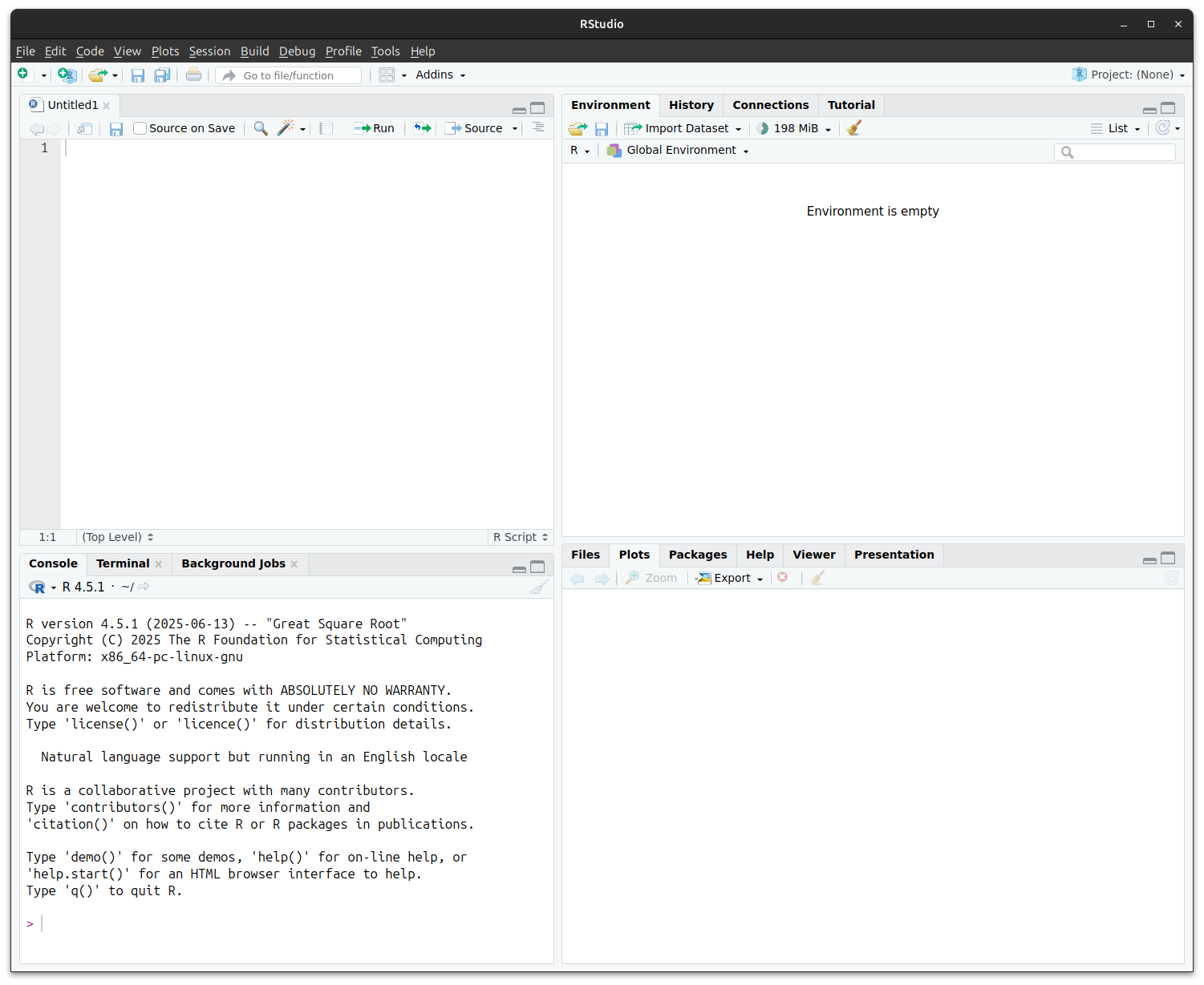
RStudio interface
RStudio is a user-friendly interface for working with R. It brings together:
- Editor: where you write and save your code.
- Console: where you run commands and see results immediately.
- Environment: where you can see the data and objects you’ve created.
- Tabs for files, plots, packages, and help, all in one window.
The RStudio environmnet lets you see your code, files, output etc. all together:
Putting it together
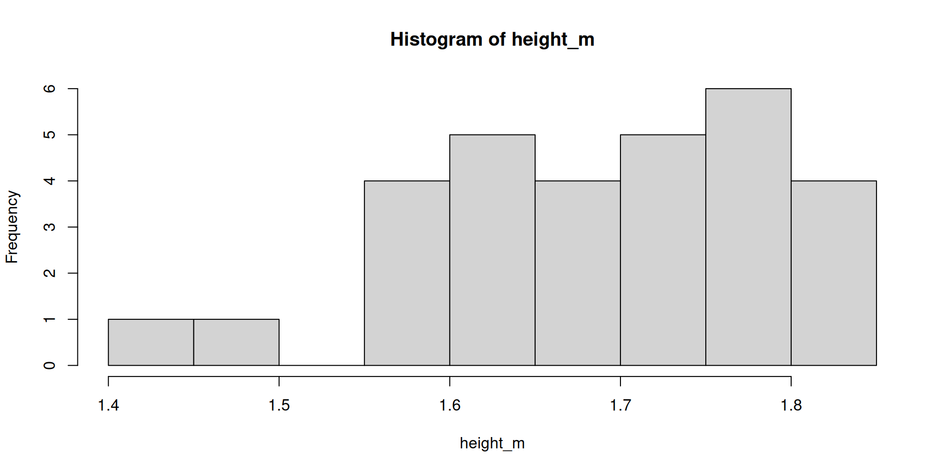
Let’s look at a simple example of how these are used. Here’s an example data set, where we recorded the heights of a sample of 30 students in an undergraduate degree programme:
We can calculate the mean and standard deviation (SD) of like so:
The mean and standard deviation of student heights is 1.69±0.10 m.